Introduction
Logistic regression is an exciting bit of statistics that allows us to find relationships in data when the dependent variable is categorical. On account of this, it has captivated the minds of many a statistician to such a degree that my school uses it to help them predict A-Level grades.
In this article we will discuss a simple binary (only outputs “yes” or “no”) implementation of logistic regression in Visual Basic and use it to make predictions based on data in spreadsheets.
Background
Super Important Terms
Hypothesis – how we predict something works (eg. “I hypothesise that the relationship between height, age and weight is given by the function w = 5h + 2a + 1”).
Parameter Vector – The vector containing what are effectively the coefficients for your hypothesis (eg. 5, 2 and 1 are contained in the parameter vector for the previous weight-height model). They are, for some reason, represented with the Greek letter θ.
Feature – a measurable property of a phenomenon being observed (eg. height and age are the features in the previous weight-height model).
Likelihood – The probability of getting a certain dataset using a certain hypothesis given a certain parameter vector.
Posterior Probability – The probability of getting a certain hypothesis with a certain parameter vector given a certain dataset.
How does one go about turning a parameter vector and values into a hypothesis?
With ease.
Using the weight predictor as an example, let  and
and  .
.
We want to get w = 5h + 2a + 1. Hmm.
If we multiplied each element in x by their corresponding element in θ, we’d get
h(x) = 1*1 + 5*h + 2*a
Put in a more abstract way, with  and
and  , our hypothesis is
  .
.
This can be done with a for-loop or, if you’re feeling extra sneaky, matrix multiplication (xTθ).
How does one go about turning hypotheses into predictions?
Now that we have a hypothesis we need to make predictions – we need to find some sort of function that maps h(x) to some value between 1 and 0 (“yes” and “no” respectively). It just so happens that a certain mathematician, Pierre François Verhulst by name, came up with exactly such a function while he was studying population growth: the standard logistic function (also called a “sigmoid” function because it looks like an “s”).

We simply pass in our hypothesis and get out a prediction. If the function is unsure, it’ll return a fraction: 0.9 means it’s pretty sure that it’s got a 1; 0.4 is a less sure 0.
Wait a second, how do we get the values for θ?
Assuming that we have example data to train with, we are now faced with an optimisation problem: to find values for θ that minimise the error in our predictions (thus optimising our model). The problem can be broken up into two parts:
Part 1: How wrong are we?
For each vector θ, we need to work out how wrong the model based upon the values is. The error metric we’re going to use is the negative log likelihood.
We define it thus:

The graphs for these cases are shown below.
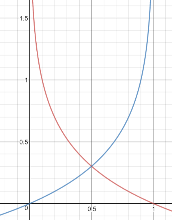
Where the red line shows  . We can see that the functions have asymptotes at x = 0 and x = 1 and that they strongly penalise wrong predictions with made high certainty (when y = 0 but we predicted something like 0.9). We can combine the expressions thus:

Where N is the number of examples in x, yi is the ith value in y and xi is the ith example in x.
Note that when yi = 0, the first term in the sum reduces to 0; when yi = 0, the second term reduces to 0. We take a log transform to make the function easier to handle – small numbers that might experience underflow become less small; multiplication becomes addition. A very good derivation can be found here: http://www.robots.ox.ac.uk/~az/lectures/ml/2011/lect4.pdf.
Part 2: How can we stop being wrong?
To stop being wrong we have to minimise the errors we make. One of the most intuitive methods of doing this makes use of elementary calculus. The negative log likelihood function for logistic regression can be shown to be concave – that is that there exists a single global optimum.
We thus take partial derivatives for all θ, multiply them by a learning rate (step size) α and then subtract them from their respective original values: where f represents a certain feature. Looping over many times, this essentially moves us closer to the optimum – like a skateboarder rolling down a valley – where  for all θ.
In the case of our logistic function, the derivative can be easily obtained from the chain rule:
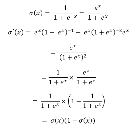
We thus arrive at the following update function:

Where f is a feature, α is the learning rate and xi [f] is the value of feature f in example xi.
In summary, our algorithm takes the following form:
Repeat for all features:
If gradient is within reasonable threshold, then exit loop
Optimising the Optimiser
We can see that convergence slows down as we approach the optimum. This is because the partial derivatives begin to near 0 and the step sizes become very small. We can counteract this by making the following tweaks to the algorithm:
- Record the squared partial derivatives for each feature in an array
 .
. - Divide the learning rate for each feature by the square root of the sum of the last 10 partial derivatives.
This dynamically changes the learning rate as we approach convergence.
We can speed up convergence further by normalising all the features. We could also take a stochastic approach by updating the parameter vector after every training example we go over though this converges “less”.
Need even more speed?
Use a different algorithm but remember: inverting matrices is effort. Newton’s method is pretty easy to do with a decent linear algebra library.
Using the code
CSV data is loaded into using the Load() method. The data should have headings in the top row.
Load("path/to/my_file_name.csv")Our logistic function and error cost function are implemented below.
 Copy Code
Function LogisticFunction(x)
    'Compute the value of the logistic function given input x
    'a sigmoid function has an S shape and is given by 1/(e^(-t))
    'e = 2.71... (Euler's number)
    Return (1 / (1 + Math.Exp(-x)))
End Function
Function LogisticCost()
    Dim cost As Double
    'Loop through all the training examples
    For i = 0 To exampleCount - 1
        Dim exampleCost As Double
        If exampleOutputs(i) = 0 Then
            exampleCost = Math.Log(1 - LogisticFunction(Hypothesis(exampleInputs(i))))
        Else
            exampleCost = Math.Log(LogisticFunction(Hypothesis(exampleInputs(i))))
        End If
        cost += exampleCost
    Next
    'Take average
    cost *= -1 / exampleCount
    Return Math.Abs(cost)
End Function
And our optimisation algorithm is implemented here:
 Copy Code
Sub Minimise()
    'Simple implementation of adagrad bc no way in hell am I implementing bfgs or anything that requires the hessan
    'gradient = X'(h(x) - y)
    Dim learningRate As New List(Of Double)
    Dim derivative As New List(Of Double)
    Dim pastGradientSquares As New List(Of List(Of Double))
    Dim sumOfPastGradientSquares As New List(Of Double)
    'Initialise all the variables
    For i = 0 To featureCount
        derivative.Add(1)
        learningRate.Add(0.01)
        sumOfPastGradientSquares.Add(0)
        pastGradientSquares.Add(New List(Of Double))
    Next
    lastCost = LogisticCost()
    deltaCost = 100
    'Do this until we converge (the derivative = 0ish)
    While (Math.Abs(deltaCost) > desiredDelta)
        Dim difference As New List(Of Double)
        Dim h As New List(Of Double)
        'Reset the derivative
        For i = 0 To thetas.Count
            derivative(i) = 0
        Next
        'Loop through the hypotheses and populate the list h
        For i = 0 To exampleCount - 1
            h.Add(LogisticFunction(Hypothesis(exampleInputs(i))))
        Next
        'Get the difference
        For i = 0 To exampleCount - 1
            difference.Add(h(i) - exampleOutputs(i))
        Next
        'Multiply by the features
        For i = 0 To exampleCount - 1
            For j = 0 To featureCount - 1
                derivative(j) += difference(i) * exampleInputs(i)(j)
                'Update the list of previous squared derivatives
                pastGradientSquares(j).Add(Math.Pow(derivative(j), 2))
                'If we exceed 10 things, just remove the oldest entry
                If pastGradientSquares(j).Count > 10 Then
                    pastGradientSquares(j).RemoveAt(0)
                End If
                'Update the sums
                sumOfPastGradientSquares(j) = Sum(pastGradientSquares(j))
            Next
        Next
        'Multiply by Learning Rate for this specific feature and get new thetas
        For i = 0 To featureCount - 1
            thetas(i) -= (learningRate(i) / (Math.Sqrt(sumOfPastGradientSquares(i) + 0.00000001))) * derivative(i)
        Next
        Dim currentCost = LogisticCost()
        deltaCost = currentCost - lastCost
        'We need to look like we're doing something so here's something to keep users occupied
        Console.WriteLine("Training...  " + LogisticCost().ToString + " " + derivative(0).ToString) ' + " " + derivative(1).ToString + " " + derivative(2).ToString)
        lastCost = currentCost
    End While
End Sub
We can quickly get predictions like this:
Function Predict(x)
    Return LogisticFunction(Hypothesis(x))
End Function
And see how well our classifier is doing like this:
 Copy Code
Sub Check()
    Dim correctlyClassified As Double = 0
    'Loop through results and see how many were classified correctly
    For i = 0 To exampleInputs.Count - 1
        Dim result As String
        If Predict(exampleInputs(i)) > 0.5 Then
            result = "Positive"
            If exampleOutputs(i) = 1 Then
                correctlyClassified += 1
            End If
        Else
            result = "Negative"
            If exampleOutputs(i) = 0 Then
                correctlyClassified += 1
            End If
        End If
        Dim trueClassification As String
        If exampleOutputs(i) = 1 Then
            trueClassification = "Positive"
        Else
            trueClassification = "Negative"
        End If
        Console.WriteLine(result + " and was actually " + trueClassification)
    Next
    Console.WriteLine("Correctly Classified " + correctlyClassified.ToString + " out of " + exampleInputs.Count.ToString)
End Sub
Demo
The classifer was trained on made-up data to model some real-life situations. Using the below data, a model was built to predict car crashes based upon wheel drive, age of car and weather conditions.
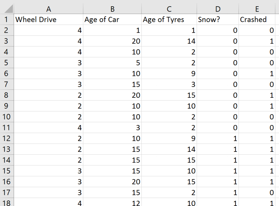
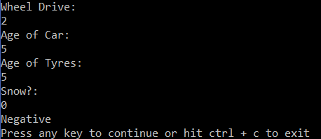
The resulting predictions looked a bit like this:
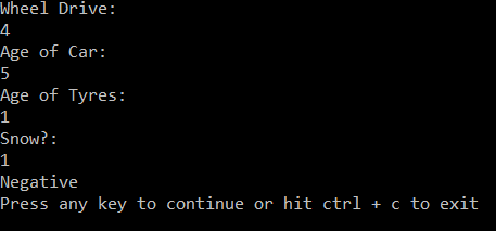
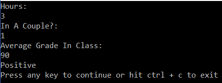
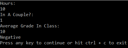
Another dataset was used to predict whether pupils would pass their exams based upon the hours they spend studying, their previous performance and whether or not they’re in a relationship.
The resulting predictions were:
Other Things to Look Into
Reguarlisation
Sometimes our models may over-fit the data. That’s a bad thing because although it might be better at classifying the training set, it may become less suitable at making predictions with new data. Reguarlisation allows us to stop it.
Multiclass classification
Classifying things into more than just “Positive”s and “Negative”s. This can quite crudely be done by creating a classifier for each class, passing your input through all of them and then choosing the highest-scoring classification.
For instance, with three classes cat, dog and table, an image of a cat might score 0.9 on the cat classifier, 0.4 on the dog classifer and 0.001 on the table classifier. We then select the classifer with the 0.9 score and return”it’s a cat”.
Source
https://github.com/PeterTheHe/VBML
History
Keep a running update of any changes or improvements you’ve made here.
- Peter the Mentor, age 16
Also published on Medium.
